Why Your A/B Test Won’t Measure That Policy Change

The marketing director walks into a planning meeting on Monday with a proposed packaging change for the company’s flagship product. The proposed change is meaningful: new label, new claim, updated brand mark, slight redesign of the bottle shape. The engineering team’s first response is to run an A/B test. Half the units ship with the new packaging, half ship with the old, the company measures the sales lift on the treated half and decides whether to roll out company-wide.

The marketing director listens to the proposal and points out that this is not how packaging changes get rolled out. Either every unit on every shelf has the new packaging in week one, or no unit does. The retail channel does not accept a mixed shipment. The shopper expectation does not accept a mixed shelf. The regulatory filing applies to a single packaging spec, not two simultaneously. The A/B test cannot run for structural reasons that have nothing to do with statistics. The packaging change is going to roll out to 100% of the customer base on a single date, and the company is going to find out the impact only after the rollout has happened.

This is the situation I have seen at every consumer business that makes policy decisions of any size: pricing rules, packaging changes, shipping policy changes, loyalty-program rule changes, return-policy changes, channel-allocation changes. A/B testing is the engineering reflex; A/B testing is the wrong tool for these decisions; the team’s analytic methodology does not yet have a replacement, so the company makes the change blindly and argues about the impact for the next two quarters using before-and-after comparisons that are systematically biased. This article is the replacement methodology: interrupted time-series analysis with intervention modeling for the average effect, and tree-based methods for the heterogeneous effect across customer segments. The methodology is forty years old and well-validated; it is under-used because most analytics teams were trained on randomized testing and were not taught the alternative.

The companion article Causal Inference Without an RCT walks through the full toolkit including synthetic controls, regression discontinuity, and instrumental variables. This article is specifically about the two methods most relevant to a policy-change decision: ARIMA intervention modeling, which gives you the average treatment effect when randomization is not available, and classification-and-regression-tree analysis, which surfaces which customer segments responded differently to the change. The two methods together produce a defensible policy-impact estimate that the executive team can act on. The remainder of this article is how to run each method and how to combine them.

Three reasons A/B testing is not available

Before reaching for an alternative methodology, the team should be clear about why A/B testing was not available for the specific decision. The answer determines which alternative is appropriate and what the inferential strength is going to be.

Legal or regulatory impossibility. Some policy changes have to be applied uniformly because uneven application would violate consumer protection rules, antitrust rules, or contractual obligations. Price changes in regulated categories (some food, some financial services, some utilities), terms-of-service changes, and privacy-policy changes typically fall into this category. The company is legally bound to a uniform rollout. The A/B test is not available; the time-series methodology is the replacement.

Ethical or reputational impossibility. Some changes affect customer welfare directly and the company would not want to apply a worse treatment to a randomized subset. Pricing increases on essential products, changes to refund policies, changes to safety-related product specifications, and changes to customer-data handling typically fall into this category. The company could legally run an A/B test but the reputational cost of being known to have run one would exceed the analytic value of the result. The time-series methodology is appropriate.

The three reasons compound. A packaging change may be operationally impossible to A/B test, regulatorily uniform, and reputationally fraught all at once. The cleaner the team is about which of the three is binding, the cleaner the methodology choice that follows.

Interrupted time series: the right tool when randomization is impossible

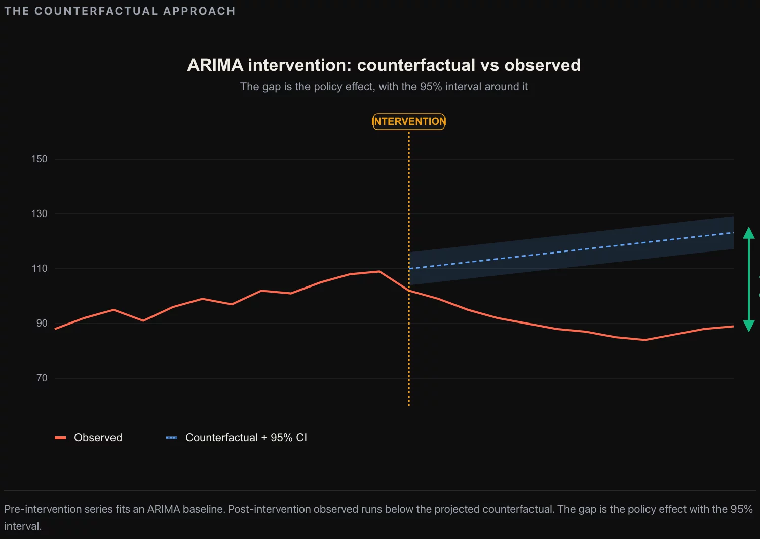
Interrupted time-series analysis is the methodology that answers the question “what is the average effect on the time-series of the population, given that we changed the policy on a specific date.” The methodology has a strong academic pedigree (Box and Tiao 1975 is the canonical reference; Campbell and Stanley 1966 framed the design as a “quasi-experiment of an interrupted time-series”). The intuition is straightforward: you fit a model to the pre-intervention time series, project that model forward into the post-intervention period, and the gap between the projected series and the actual series is the policy effect.

Step 1: assemble the time series. Pull the outcome metric at a regular cadence (daily, weekly, or monthly depending on the policy and the noise level) for at least 36 months prior to the intervention and at least 6 months after. The longer the pre-period, the better the baseline fit; the longer the post-period, the more robust the effect estimate.

Step 2: identify the ARIMA order. Fit an ARIMA(p,d,q) model to the pre-intervention period only. Use the autocorrelation and partial-autocorrelation functions to identify reasonable values for p (autoregressive order), d (differencing order), and q (moving-average order). In most consumer demand series, the right model is ARIMA(1,1,1) or ARIMA(2,1,1) with seasonal differencing for monthly data. Verify the fit by checking the residual autocorrelation and the Ljung-Box test on residuals.

Step 3: specify the intervention function. The intervention can be modeled as a step (the policy change creates a permanent level shift), a pulse (the policy change creates a one-period spike that fades), a ramp (the effect builds gradually over a few periods), or a combination. For a price increase, the step function is usually right. For a regulatory change with a phase-in period, a ramp is appropriate. For a one-off campaign or event, a pulse with a decay term is appropriate. The choice of intervention function is the most consequential modeling decision and it should be made before looking at the post-intervention data.

Step 4: fit the full model. Refit the ARIMA model on the full series (pre and post) with the intervention function included. The coefficient on the intervention function is the estimated effect. The standard error on the coefficient produces the confidence band. The methodology is identical to the classical ARIMA estimation in any production statistics package.

Step 5: validate the model. Check the residuals on the full series. They should be approximately white noise. If the residuals show structure (autocorrelation, heteroscedasticity, trend), the model is misspecified and the intervention coefficient is biased. The fix is to add structure to the ARIMA component, not to the intervention component.

Step 6: report the effect with its assumptions. The estimated effect is a number with a confidence band, conditional on the ARIMA model being well-specified, the intervention function being correctly chosen, and the only thing that changed at the intervention date being the policy under study. The third assumption is the one that breaks most analyses; the next section is about how to defend it.

The output of the methodology is a single number: the estimated average effect on the outcome metric, with a 95% confidence band. For a packaging change that was estimated to be revenue-neutral at the planning meeting, the output might be “the change produced a +1.8% lift in monthly category revenue, 95% CI [+0.4%, +3.2%].” That number is what the executive team makes decisions on going forward.

Defending the assumption that nothing else changed

The interrupted-time-series methodology is only as good as the assumption that the intervention is the only thing that changed at the intervention date. In practice this assumption is rarely strictly true. Three patterns are worth checking:

Concurrent changes. Other policy changes, market events, competitor moves, or seasonal effects may have happened at or near the intervention date. The fix is to extend the pre-intervention period back far enough to absorb the typical seasonal pattern, and to explicitly model any other identifiable concurrent change as a separate intervention function. If a competitor launched a new product in the same week as the company’s packaging change, both events go in the model and the coefficients are estimated jointly. If a regulatory change took effect in the same quarter, it gets its own intervention function. The model can accommodate up to three or four concurrent interventions before the identification becomes weak.

External time series as comparison. Where available, include an external time-series that is similar to the company’s outcome but should not be affected by the intervention. For a company-specific packaging change, the category-level revenue (from public retail trade data or a syndicated audit) is a natural comparison. The model becomes a difference-in-differences within the ARIMA framework: the company’s series and the comparison series both have ARIMA structure, and the intervention is estimated on the difference. This dramatically tightens the confidence band when a good comparison series is available.

Sensitivity to model specification. Refit the model with different ARIMA orders (e.g., ARIMA(1,1,0), ARIMA(2,1,1), ARIMA(1,1,2)) and different intervention specifications (step vs. ramp vs. pulse). If the estimated intervention effect is stable across reasonable specifications, the methodology is well-grounded. If the estimated effect varies by more than 30% across specifications, the result is fragile and the report should acknowledge it.

The three checks are what turn a “we think the packaging change added 2%” estimate into a “the packaging change added 1.8% with 95% confidence [0.4%, 3.2%], robust to the comparison series we tested and to four alternative model specifications” statement. The first version of the statement is dismissible. The second version is decision-grade.

What CART tells you that the average effect does not

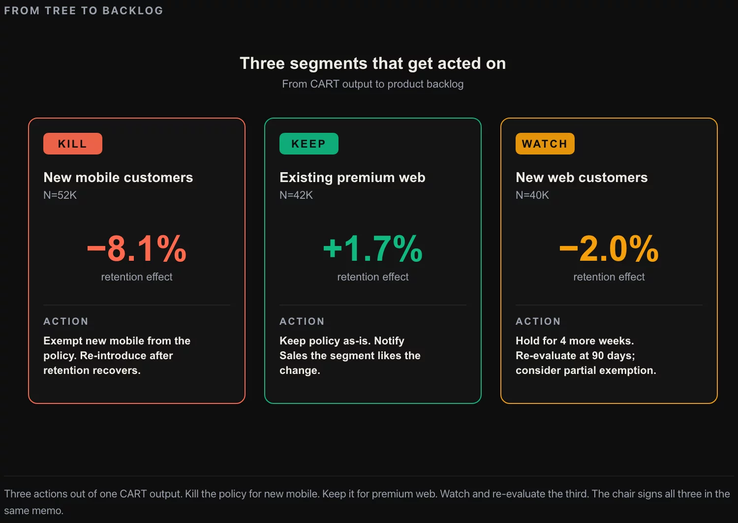
The interrupted-time-series methodology produces an average effect. The average is a useful first-order answer; it is rarely the right answer for executive decision-making, because the average effect typically hides meaningful heterogeneity across customer segments. A policy change that produces +1.8% average revenue might be +6% for high-tenure customers, +0.4% for new customers, and negative for one specific segment that the company would have wanted to know about before rolling out.

The technical recipe is four steps.

Step 1: define the target variable. Pick the customer-level outcome the policy was supposed to affect: revenue per customer, basket size, purchase frequency, retention. The target should be measurable at the customer level both before and after the intervention.

Step 2: assemble customer features. Pull the customer attributes that might explain variation in the response: tenure, total historical spend, category mix, channel preference, geography, recency, frequency, monetary segments. Twenty to forty features is the typical range; more features make the tree fit noise.

Step 3: fit the tree on the pre-intervention period. Use the pre-intervention data to build the tree that best explains variation in the outcome under the previous policy. Use pruning to prevent overfit: ten-fold cross-validation, prune the tree back to the depth where the cross-validated error stops improving. The tree will typically have between 8 and 30 leaves.

Step 4: apply the tree to the post-intervention period. Assign each post-intervention customer to a leaf using the tree from the pre-period. Compute the average outcome inside each leaf for the post-period. Compare to the pre-period average for the same leaf. The difference is the leaf-specific intervention effect. Identify the leaves where the effect is meaningfully different from the average.

The output is a decision tree with a number on each leaf: the policy effect for the customers in that leaf. The executive team reads the tree, identifies the segments where the policy worked, the segments where it did not, and the segments where it caused harm. The next quarter’s work is the segment-specific adjustment: rule changes, communication, retention offers, channel-specific pricing.

The classical limitation of CART is that the tree is unstable: a small change in the training data can produce a very different tree. The fix in current methodology is to use a causal forest (a random-forest variant designed specifically for treatment-effect estimation, introduced by Wager and Athey in the 2010s) instead of a single tree. The causal-forest output is a per-customer estimate of the treatment effect, which can then be aggregated into segments using a separate decision tree fit to the per-customer estimates. The methodology is well-supported in production statistical packages; the additional complexity is worth it when the policy decision has segment-specific implications.

Three traps in post-policy measurement

Three patterns that catch first-time practitioners and produce wrong policy-effect estimates. Each one is addressable; the three together are why most post-policy measurement programs ship results that have to be retracted six months later.

Trap one: cherry-picking the comparison period. The default before-and-after comparison takes the three months before the policy and the three months after, and reports the difference. The result is highly sensitive to the choice of three months. The fix is to use the full ARIMA model and to report the intervention coefficient with its confidence band, not a point estimate of the before-and-after gap. The three-month-window comparison is fine for an internal first-look; it is not fine for a decision the company is going to act on.

Trap two: regression to the mean. If the policy was rolled out in response to a measured problem (declining revenue, declining conversion, declining retention), the pre-intervention period probably captures a temporary downward fluctuation that would have reverted naturally even without the policy change. A naive before-and-after comparison attributes the natural reversion to the policy, inflating the estimated effect. The fix is to use a long enough pre-intervention window (24 to 36 months) that the regression to the mean is absorbed into the baseline, and to fit the ARIMA model on the full pre-window rather than a recent subset.

Trap three: confounded segment-effect interpretation. The CART tree identifies leaves where the post-intervention outcome was different. The interpretation is “the policy had a differentiated effect on these segments.” The alternative interpretation is “these segments were also affected by something else that happened around the same time as the policy.” The fix is to look at the pre-intervention trend for each leaf: if a leaf was already on a different trajectory than the average before the policy, the post-intervention difference may not be the policy’s effect. The discipline is to read the tree alongside the pre-period trajectory for each leaf, not to read the tree alone.

The three traps compound. A team that picks a short comparison window, ignores regression to the mean, and reads the CART tree without checking pre-period trajectories will produce an effect estimate that is biased upward by every one of the three mechanisms, and the bias will not be visible from the analysis output. The discipline is the methodology; the methodology only works if it is applied with the diagnostics.

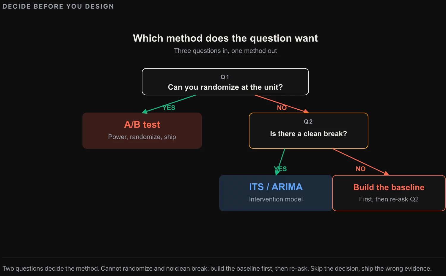
When to use which methodology

A simple decision tree for the practitioner: if randomization is available, use it. If randomization is not available and the question is “what is the average effect,” use ARIMA intervention modeling. If the question is “what is the differential effect across segments,” use CART or causal-forest on the post-intervention data, with the intervention-period assigned by the date of the change. If the question is both, use ARIMA for the average and CART for the segmentation, and report both numbers with their respective confidence statements.

The most common error in practice is to use the wrong methodology for the question, not to use the methodology badly. A team that uses a t-test on before-and-after means is asking the right question with a methodology that does not control for autocorrelation, seasonality, or trend, and the answer is biased in directions that depend on the specific data. The fix is not to fix the t-test; the fix is to use ARIMA. A team that fits a CART tree without considering the policy as the intervention is asking a different question (what explains variation in the outcome under the current policy) and is going to get an answer that the executive team will misread as a policy-effect statement.

What to do this week

If you are about to roll out a policy change and want to know how to measure its effect, three actions before next Tuesday.

Pull the time series for the outcome metric the policy is supposed to affect, at the finest cadence the data supports, for the last 36 months. Plot it. Look at it. If the series has obvious seasonality, the methodology needs seasonal terms in the ARIMA. If the series has a clear trend, the methodology needs differencing. If the series has structural breaks unrelated to the policy under study (a previous policy change, a competitor event, a market shock), those breaks have to be modeled as separate interventions. The plot tells you all of this in fifteen minutes and tells you whether the methodology is well-suited to your data or whether you have additional modeling work to do first.

Identify the customer-level features you have available for the segmentation analysis. If you cannot link the outcome metric back to individual customers, the CART step is not available and you only get the average effect; this is a data-architecture problem that the next quarter’s work should fix. If you can link the outcome back to individual customers, draft the feature list (tenure, geography, channel, category mix, recency, frequency, monetary) and verify each feature is available at the same level of granularity as the outcome.

Pick the intervention date and the intervention function specification before the rollout happens. Document them in a one-page memo that the analytics team signs off on. The discipline is to commit to the methodology before the data is in. A team that decides on the methodology after seeing the post-intervention data is producing a result that has been implicitly selected for, and the result will not survive a methodological review.

Three actions, two afternoons. They do not produce the measurement. They produce the conditions under which the measurement will be defensible. In my experience the diagnostic that matters most is the third: a team that has committed to the methodology before the rollout produces results that the executive team can act on, and a team that retrofits the methodology to the data produces results that fall apart on close inspection. The methodology is forty years old. The discipline of using it correctly is what makes the difference.