Color Palettes for Data Viz: What Survives a Client Deck

Most of the “fix our dashboard” engagements we take on start with the same observation: the analysis is fine, the chart logic is fine, the deck looks amateur. Eight out of ten times the fix is color. Not “more color” — usually less. Not “brand color” — usually a brand color that’s been pushed past where it’s useful. This article is the working set of color decisions we apply when rebuilding a client dashboard before it goes to an executive.

It is not a comprehensive theory of color. The single best long-form on that is still Lisa Charlotte Muth’s “How to pick more beautiful colors for your data visualizations” on the Datawrapper blog, written in 2018 and still the best 30 minutes you can spend on the topic. We use that essay as house reading on our team. What follows here is more specific: the calls we make in client work and the trade-offs we balance against, not a textbook.

The vocabulary that lets you fix things instead of guessing

Picking colors in RGB or HEX without HSB is like debugging a query without EXPLAIN. You can swap values around hoping it improves, but you can’t say what’s wrong.

The three coordinates you actually need:

• Hue — position on the color wheel, 0–360°. Red ≈ 0°, orange ≈ 30°, yellow ≈ 60°, green ≈ 120°, blue ≈ 240°.
• Saturation — 0% (gray) to 100% (maximum chroma).
• Brightness / Value — 0% (black) to 100% (the color itself).

HSL and HCL are siblings (HCL is perceptually-tuned, matters more for sequential gradients than for picking categorical swatches). For day-to-day work, knowing the HSB triple of any color is enough to diagnose what’s wrong.

When a teammate says “the green is too loud,” we usually mean the S value is too high. “The chart is tiring” usually means B is too high across the board. Naming the dimension makes the fix mechanical instead of vibes-based.

The four scenarios that cover most charts

Almost every coloring decision we make falls into one of four buckets. Get the bucket right and the rest is small.

1. Categorical, ≤5 series. A bar chart with five regions, a line chart with five products. Pick from one neighborhood of the wheel and vary saturation/brightness.

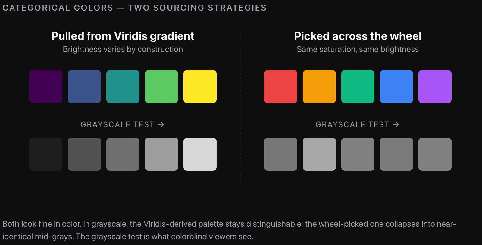
2. Categorical, 6–10 series. Don’t free-hand it. Sample from a perceptually-uniform gradient (Viridis, Inferno, Magma, Cividis) at evenly-spaced stops. Every color is guaranteed to have a different brightness, so the chart still parses in grayscale.

3. Sequential / ordinal. One hue, ramp brightness. Use Datawrapper / matplotlib / Tableau built-ins; don’t roll your own. ColorBrewer is still the gold standard.

4. Brand-constrained. Client’s brand red is mandatory. Pin it as the highlight; build the rest of the palette as desaturated neutrals around it. The brand color becomes a focus marker, not a category color.

Most “kindergarten box” dashboards we inherit are case 1 done as case 2 — five categories pulled from across the wheel because the analyst confused “I have five categories” with “I need five different hues.”

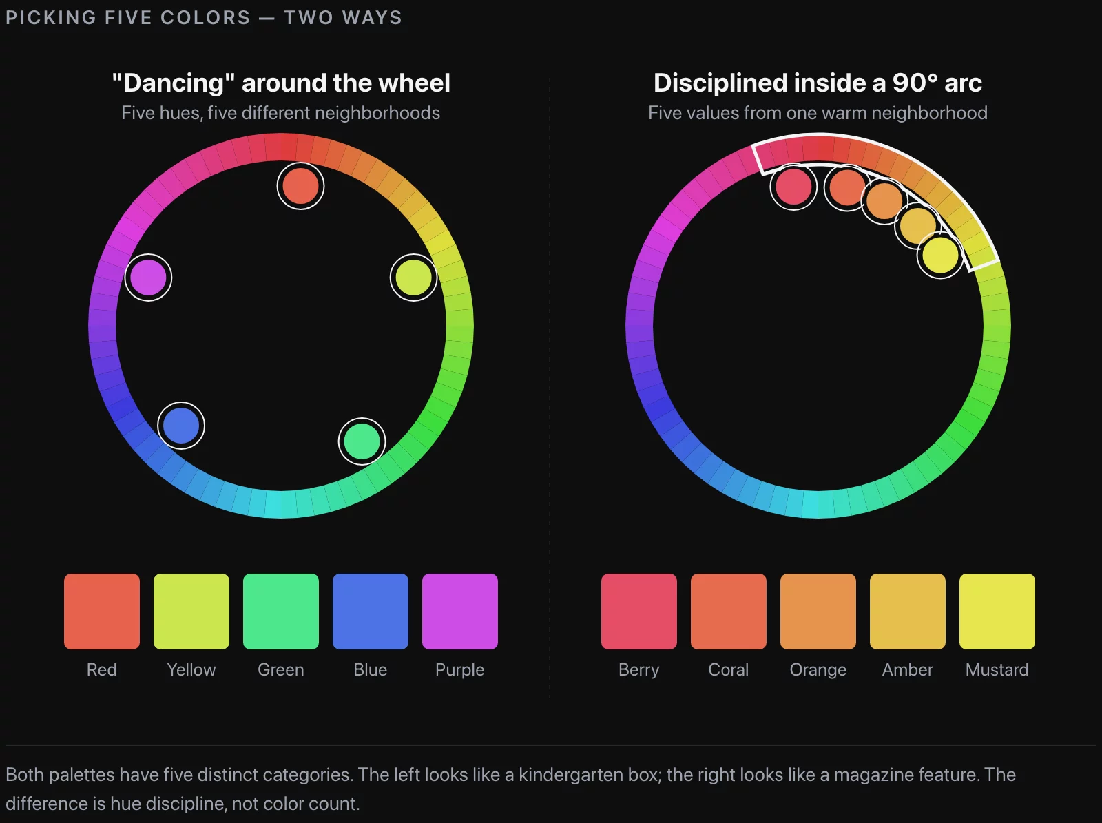
Stay in a neighborhood

In a five-series chart, the temptation is one hue per series — red, yellow, blue, green, purple. The result feels like a chart drawn for a classroom. There are thousands of usable colors inside any 60° wedge of the wheel; you don’t need to walk the whole 360.

The fix is mechanical: pick a starting hue, stay within 60–90° of it, and let saturation and brightness do the heavy lifting. A warm-amber and a coral are both inside the same wedge and read as two distinct categories. Drop saturation on one, bump brightness on the other, and you have two categories without ever crossing into the green section.

Tools that make this easier:

• Adobe Color (color.adobe.com) — analogous and monochromatic modes stay inside neighborhoods.
• Coolors.co — fast iteration on whole palettes; locking colors and reshuffling is faster than picking by hand.
• Paletton — sliders that let you shrink the angle between picks until they snap.

The “tetradic” or “square” mode in any of these is a trap; it returns four hues evenly spaced around the wheel, which is the kindergarten box.

The combination that does most of the work: warm + blue

If we had to pick one palette family that ships on more client dashboards than any other, it’s yellow / orange / red on one side, blue on the other. It’s what The Economist defaults to, what Reuters Graphics defaults to, and what we default to maybe 70% of the time.

Three reasons we keep coming back to it:

• Internal contrast. Yellow, orange, red sit close enough to feel like a family but stay distinct. You get up to three categories from one slice of the wheel.
• Blue absorbs anything. Dark, light, washed, saturated — blue reads as “calm professional” across a wide range of values. You can move blue around without breaking the chart.
• Colorblind safety. Red-green is the common deficiency (~8% of men, ~0.5% of women). Orange-blue is the safest two-category palette there is.

The only constraint where this fails is brand red: if the client’s red is a hard requirement and they want it next to green for “good vs. bad”, you have to either fight that or color-code by something else.

Green is the hardest color to use right

Pure 120° green — what you get if you type green in CSS — is dark when saturated and turns neon when you brighten it. It’s also the worst color to put next to red.

The pattern we use, lifted directly from newsroom practice: shift the hue toward yellow (down to ~80°) or toward blue (up past ~160°). Almost every “green” in a polished modern chart is actually yellow-green or blue-green, sitting somewhere in the 90–110° or 150–170° range. The Washington Post and The New York Times run greens at around 14% saturation pulled off pure 120° — distinctly green to the eye, not fighting the rest of the palette.

If a chart genuinely needs two greens, use one yellow-leaning and one blue-leaning. They read as two distinct categories without the reader thinking “the designer ran out of colors.”

Equalize loudness — then break it on purpose

Every color in a chart pulls some amount of weight from the reader’s eye. If they don’t all pull equally, the chart accidentally tells the reader which series matters most. Sometimes that’s the goal; usually it’s a bug.

What makes one color “louder” than another:

• Higher saturation
• Closer to a pure point on the wheel (0°, 60°, 120°, 180°, 240°, 300°)
• Higher contrast against the chart background

When you want categories to feel equal, equalize on these. When you want to highlight one series, deliberately leave it brighter and more saturated, and desaturate everything else into gray-blue or gray-orange. We use this pattern constantly: a single bar in coral against a row of muted bars is the most powerful “this is the one to look at” affordance in dashboard design.

The check we run before shipping: take a screenshot, run it through a grayscale filter. If categories are still distinguishable in gray, the brightness ladder is doing the work. If they collapse, the chart leans entirely on hue and will fall apart for any colorblind viewer.

Pure colors and 100/100 palettes look like a warning sign

Two specific things make a chart feel aggressive instead of informative:

1. Pure colors. A color sitting exactly on a 60° tick on the wheel (or where two of its RGB values are identical) feels intense in a way that’s distracting. The fix is a small nudge: shift the hue 5–10° off the pure point, or drop saturation by 10%. The “vivid red” you actually want is at 5° or 355°, not 0°.

1. 100% saturation + 100% brightness. This is the neon palette — the one that screams. There’s evidence from the data-viz literature (Bartram, Patra & Stone, CHI 2017, Affective Color in Visualization) that highly-saturated, highly-bright colors communicate “alarm,” not “trust.” If your dashboard is a status overview, alarm is the wrong default.

You’ll see neon palettes on big-publication interactives and think the rule is wrong. Look closer: those colors look bright but are usually 10–20% off pure brightness or saturation. Take a grayscale screenshot of the NYT music chart and the colors fall into distinct shades. Take one of an actual neon chart and it collapses to one gray.

Backgrounds: match the palette or vice versa

A surprising amount of “the palette looks weak” feedback traces to background mismatch.

For light (near-white) backgrounds:

• Avoid colors with brightness > 95% and saturation < 7%. A pastel coral on white at 1px line width disappears.
• Heavy dark-saturated colors make the chart feel ink-heavy and panicked.

For dark backgrounds:

• Drop saturation. A 78%-saturated coral that reads beautifully on a #0e0e0e dark theme looks aggressive on white at the same values.
• Keep brightness in the 10–25% range for chart elements. Pure-black-on-pure-black gives you no contrast to lift off the background.

For the v2 theme on valiotti.com, our background is #0a0a0a and the default coral is #ff694d. On the same site in a light theme we’d drop the brightness on that coral to around 60% and keep the hue the same.

A colored chart background — anything other than near-white or near-black — costs you in two ways: it pulls attention from the chart, and every category color now competes with the background. We avoid tinted chart backgrounds unless the design brief explicitly calls for them.

When you’re stuck, copy

There is no shame in cribbing palettes from sources that already work. The mistakes that look amateur in client decks are almost never mistakes of taste — they’re mistakes of starting from scratch when there are five thousand worked examples sitting in any newsroom archive.

Where we steal from:

• Newsroom graphics. The Economist, The Pudding, South China Morning Post, FiveThirtyEight. Screenshot a chart you like, eyedrop the values into Adobe Capture or image-color.com, note the HSB triples. Over time you train your eye on the S and B combinations that survive review.
• Film stills. Wes Anderson palettes are a meme for a reason; they survived a colorist. Movies have whole frames of intentional color decisions.
• Built-in palettes. Matplotlib’s tab: family (since 3.7) is a Vega-derived palette that already obeys most of the rules above. If you’re starting a Python notebook for a client, start there and only override with a reason.
• ColorBrewer. Cynthia Brewer’s palettes are still the safest categorical and sequential defaults available for free, and they ship with explicit colorblind-safety labels.

The point isn’t to plagiarize a specific palette; it’s to internalize what saturation and brightness values feel like in something that already shipped.

Modern tooling: 2026 notes

A few practical updates from five years of client work:

• Tableau ships with Viridis-family and tab: defaults. You no longer need to import anything for the common cases.
• Looker / Looker Studio default to a “Material” palette that is, in practice, warm-plus-blue with one ornamental green sitting at pure 120°. We almost always override that green to a yellow-green.
• Plotly Express defaults to Plotly (10 colors, well-behaved) — fine for prototyping but we still resample from Viridis for >5 categories.
• Matplotlib 3.7+ added the 'tab:' family as defaults. Start your notebook with tab:blue, tab:orange, tab:green and only deviate when there’s a reason.
• Storybook / Figma tokens. If a client has a design system, demand the chart palette upfront. Half our worst-looking dashboards have been the result of an analyst picking colors that contradicted the design system the marketing team had already shipped.

The general direction across all of these: defaults are getting better. The rules above bite less often than they did five years ago. They still bite when an analyst overrides a sane default with brand colors picked from a logo without HSB intuition.

A checklist for before something leaves your screen

The pre-flight we run on any chart heading to a client deck:

1. Stay inside a narrow region of the color wheel; let saturation and brightness carry the variety.
2. Default to warm + blue. Override only when a brand palette forces it.
3. If you use green, pull it yellow or blue. Avoid pure 120°.
4. Avoid pure colors (0°/60°/120°/180°/240°/300°) and 100%/100% saturation/brightness pairs.
5. Grayscale-test categorical palettes. If they collapse into one tone, swap to colors pulled from a Viridis-family gradient.
6. Equalize loudness across categories unless you’re deliberately highlighting one.
7. Match colors to background. Pastels die on white; saturated colors panic on dark.

When in doubt, copy. There is no shame in cribbing; there is shame in shipping a kindergarten palette to an executive.

Further reading

• Lisa Charlotte Muth, How to pick more beautiful colors for your data visualizations — Datawrapper, 2018. The single most useful long-form on this topic; the source we recommend to every analyst we work with.
• Cynthia Brewer, ColorBrewer 2.0 — the original colorblind-safe categorical and sequential palettes.
• Bartram, Patra & Stone, Affective Color in Visualization, CHI 2017 — the academic basis for “don’t ship neon.”
• Viridis colormap documentation — why perceptually-uniform sequential gradients matter and which to pick.