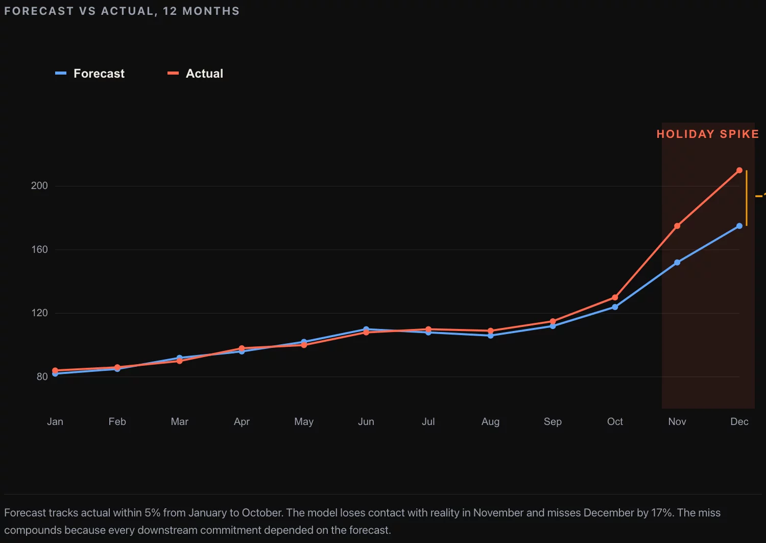
Every consumer business with a planning function has a forecast that runs eleven months a year and breaks the twelfth. The numbers are quiet from January to October, the model tracks within four or five percent of actual, the planning team builds the next quarter on it. November lands within seven percent. December lands eighteen percent below the actual print. The CFO writes a memo to the planning team about the miss. The planning team rebuilds the model. Next year the model runs quiet from January to October and the December print misses by sixteen percent. The variance has compressed. The shape of the miss has not.
In This Article
This is the failure mode I have seen at every consumer business I have walked into in the last decade. The model is not bad. The factors in the model are appropriate. The methodology is recognizably econometric and would pass a textbook review. The problem is that December is not the same kind of month as the other eleven, and a forecast architecture that treats it as a multiplier on the baseline is going to miss every year by an amount that depends on how cleanly the holiday signal happens to land that particular cycle.
The fix is a two-model architecture: a short-horizon model that handles December as its own animal, and a long-horizon model that gets the other eleven months right. The two models share inputs, share a calibration loop, and ship as one forecast with a documented confidence band that widens in December. The architecture below is the one I have built in production three times. The factor list is the one that worked for a US beverage manufacturer with a $2 billion category business and a category R² of 85%. The factors translate to any consumer category with enough history to support a regression; the methodology does not depend on the industry.
The deliverable from a fractional CDO engagement at a consumer business with a chronic Q4 forecast miss is two production models, a sensitivity table for ten factors, a calibration log that shows month-over-month errors for the last 24 months, and a one-page memo that gives the executive team the confidence band for the next 90 days of demand. The remainder of this article is the architecture that produces the memo.
Why every forecast model breaks in December
A consumer demand forecast breaks in December for three structural reasons. Each one is fixable; the three together are why no single fix has ever closed the Q4 gap by itself.
The seasonality dummy is the wrong shape. Most forecast models include twelve monthly dummies, with January or the lowest-volume month as the omitted base. The December dummy is then a constant: the average difference between December and the base, learned from history. This works in categories where the December-to-baseline ratio is stable across years. It fails in categories where the December lift varies by 8% to 20% across cycles depending on calendar position, weather, real-income trajectory, and competitive pricing. The December dummy is too crude a tool for the question being asked.
The base period is dirty. Most models fit on a multi-year window that includes the previous year’s December, the previous year’s holiday-week trough in early January, and several months of post-holiday distortion. The trend coefficient is being asked to explain a non-stationary process. The fix is to pick a base month with the smallest dispersion across years (in most consumer categories this is February, which is post-holiday-distortion and pre-spring-cyclical) and anchor the seasonality factor adjustment to that base, rather than to an annual average.
The three failure modes are why a competent econometric forecast that performs within 5% from January to October systematically misses December. Each one shows up in the residual diagnostics if you look. Most forecasts ship without anyone looking.
The two-model architecture
The fix is not to build a better single-model forecast. The fix is to run two models in parallel and use each for the horizon it is good at.
The long-horizon model is a regression with the full factor set. It is asked to forecast 12 months out, with the input factors themselves coming from external forecasts (econometric forecasts of real income, regulatory forecasts of excise tax, calendar forecasts of weather, internal planning forecasts of trade-marketing spend). The regression produces a 12-month demand path with a sensitivity table per factor. It is wrong by 10% to 30% in any single month; it is right within 4% on the annual total in a stable category. The role of the regression model is not to call the December number; the role of the regression is to size the next year, allocate the planning budget, and price the senior team’s decisions about category investment.
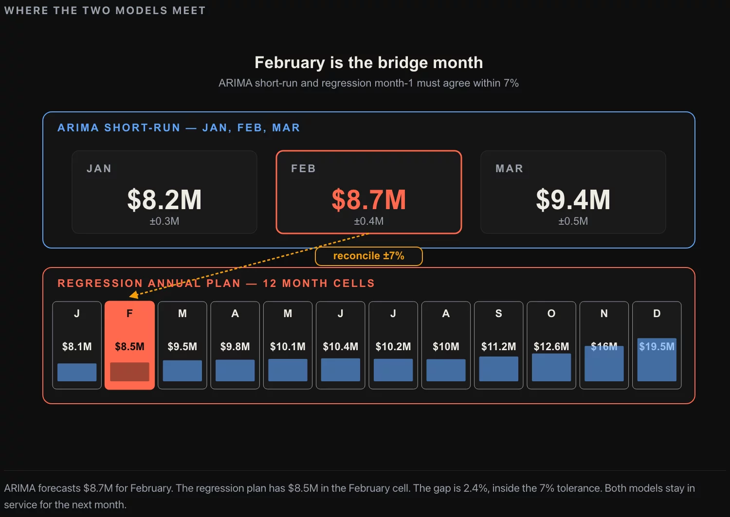
The two models reconcile at the one-month horizon. Every month, the ARIMA forecast for the upcoming month is compared to the regression forecast for the same month. If the two are within 4%, the ARIMA forecast ships. If they diverge by more than 4%, the planning team digs into which input has changed: a factor in the regression that the ARIMA does not see (a new excise tax, a competitor launch, a major weather event), or a short-term shock that the ARIMA has caught and the regression’s factor proxies have not. The reconciliation is the mechanism that catches the systematic Q4 miss before it lands.
The ten factors that actually move category demand
The factor list is not theoretical. It is the list that emerged from variable selection on three years of monthly category sales data, against a candidate set of forty initial factors. The ten that survived multicollinearity and stat-significance tests, with their sensitivity coefficients from the production model on a beverage manufacturer’s data:
| Factor | Coefficient | Interpretation |
|---|---|---|
| Average monthly temperature, YOY change | +1.0% per +1°C | Warmer month, more category demand |
| Real disposable income, YOY change | +0.5% per +1% | Income directly drives premium-tier volume |
| Modern trade spend, YOY change | +0.1% per +1% (total) | Trade promotion has small but reliable lift |
| Traditional trade spend, YOY change | +0.15% per +1% (total) | Modest channel-specific lift |
| Shelf assortment, +1 SKU point | +3.3% YOY | The single highest-leverage factor |
| Impulse-channel regulation impact | -2.0% one-time | Regulatory shifts compress volume |
| Category advertising GRP, YOY change | +1.6% per +1% (+126 GRP) | TV is still measurable, still material |
| Adjacent category volume, YOY change | +0.9% per -1% | Substitution dynamic with adjacent category |
| Adult population, YOY change | +0.8% per +1M people | Demographic base, slow-moving |
| Excise tax change, +$1/unit | -1.0% | Direct cost pass-through to consumer |
The coefficients tell the operating story. Shelf assortment is the single highest-leverage factor: a one-point gain in shelf-SKU count produces a 3.3% volume lift, more than any other input the manufacturer can directly influence. Real income matters but is exogenous; weather matters and is exogenous; advertising matters in the way regulatory-style elasticity studies say it matters; trade spend matters but at a much smaller marginal rate than the brand teams typically assume.
The factor that does not appear is competitive pricing. The first version of the model included a market-price index. It was statistically significant but collinear with category advertising; the version of the model that ships drops the price index in favor of advertising and accepts the collinearity. This is the kind of decision that has to be made consciously in the model design; the result is documented in the calibration log.
The R² on the production model with these ten factors is 85%. The remaining 15% of variance is the noise the ARIMA model is supposed to catch on the one-month horizon. Pushing R² above 85% by adding factors does not improve the one-month forecast; it overfits the historical data and makes the next December miss in a different direction.
December is not a multiplier
The single technical change that closes most of the Q4 miss is replacing the December dummy with a calendar-aware seasonality factor and adding a December-specific AR(1) term to the short-horizon model.
The calendar-aware seasonality factor takes the form: December demand = base-period demand × seasonality multiplier × calendar adjustment × external-event adjustment. The seasonality multiplier is learned from history. The calendar adjustment captures the day-of-week composition of the month (December with five weekends is different from December with four). The external-event adjustment is the place where you put the one-off factors that show up year over year: known competitor launch, major regulatory change, weather anomaly. The factor is multiplicative and each component is auditable.
The AR(1) term in the short-horizon model is the autoregression on the previous month’s residual. The intuition is that if November landed 6% above forecast, December is more likely to also land above forecast than to revert; if November landed 4% below forecast, December is more likely to under-deliver than to bounce. The AR(1) coefficient on monthly consumer category data tends to be between 0.3 and 0.6, which means a 5% November surprise carries forward as a 2% to 3% adjustment to the December forecast. This is the mechanism that produces the “December within 6%” forecast at a category business that previously ran “December within 15%”.
The MAPE on the production model for the one-month December forecast is 5% to 8%, depending on the year. The MAPE on the long-horizon regression for December is 12% to 18%. The two are not contradictory; they answer different questions. The ARIMA is the operational forecast for next month’s planning. The regression is the strategic forecast for the annual plan. The planning team works off the ARIMA. The CFO works off the regression. The two reconcile in the September planning cycle for the upcoming year.
Three traps that compound in Q4
Three failure modes in the model design that are individually survivable but compound during the holiday months. Each one is worth a separate sanity check before the model ships.
Trap one: trend coefficient absorbing seasonality. A regression on a short historical window (less than 36 months) struggles to disentangle a linear trend from a non-stationary seasonal pattern. The trend coefficient absorbs part of the seasonal effect, and the model interprets the December lift as part of a steeper underlying growth. When the next year’s December under-delivers, the model attributes the miss to the trend, which then under-forecasts the following January. The diagnostic is to plot the residuals by month and look for a December-shaped wave. If the December residuals are consistently above the others, the seasonality is undertuned and the trend is overtuned.
Trap two: collinearity between trade spend and advertising. Trade marketing spend and advertising spend tend to ramp together in Q4. Both feed into category demand. If both are in the regression, the coefficients fight each other and the model produces unstable predictions when one input changes. The fix is variable selection: keep the input with the stronger univariate correlation with demand and drop the other, accepting that some of the dropped factor’s effect is implicitly captured by the surviving factor. This is a judgment call and it should be documented.
Trap three: heteroscedasticity in the December residuals. The model’s residuals are larger in December than in March. If the model is fit by ordinary least squares without correcting for heteroscedasticity, the standard errors on the coefficients are too small and the confidence bands on the forecast are too narrow. In Q4 specifically this means the model presents a 90% confidence band of ±4% when the true 90% band is ±9%. The CFO opens the forecast, sees the narrow band, decides the forecast is high-confidence, and is surprised in January. The fix is to weight observations or to refit using weighted least squares with heteroscedasticity-robust standard errors. The math is standard; the discipline to do it is not.
The three traps compound because the model that has all three is a model that confidently presents a Q4 forecast which is mis-trended, missing the trade-vs-advertising decomposition, and showing a confidence band narrower than the actual variance. The fix is to run the diagnostics and report them to the executive team. A model that does not report its diagnostics is a model that is asking the executive team to trust it on faith, and in Q4 specifically that trust is misplaced more often than not.
Calibration log: how you know the model is working
The forecast architecture only earns the right to ship if it produces an honest calibration log: the forecast for each month, the actual print, the gap, and the explanation. The log is read every month at the planning meeting. The accumulated log over 18 to 24 months is what the CFO uses to decide how much to trust the forecast in the next planning cycle.
The log has four columns: month, forecast, actual, residual percentage. A fifth column captures the named factor that drove any residual above 5% (e.g. “weather +2.5° YoY, model implied +2.5% volume not the actual +6% — model under-weights weather extreme months”). The fifth column is the part that turns a calibration log into a learning loop. A log without explanations is just a record of misses; a log with explanations is the source of next year’s model improvement.
The discipline that makes the log work is that the forecast is locked at the start of each month and the residual is computed exactly once, at the end of the month, before the next month’s forecast is generated. The model is not rerun in the middle of the month to “incorporate new information.” The forecast for any given month is a single number, a single confidence band, and a single residual when the actual lands. The temptation to update the forecast mid-month is what produces planning teams that cannot tell whether their model is improving or not.
What to do this week
If you are running a consumer demand forecast and the last Q4 missed by more than 10%, three actions before next Tuesday.
Pull the last 36 months of monthly category demand. Plot it. Look at the November-December-January slope each year. If the slope varies by more than 5 percentage points across years, your seasonality factor is the wrong shape and the next quarter’s work is replacing the monthly dummies with a calendar-aware factor structure. The plot takes ten minutes and tells you whether the problem is in your seasonality definition or somewhere else.
Pull the residuals from your current model for the last 24 months. Plot them by month. If December residuals are systematically above (or below) the other months, your model is mis-trended, the trend is absorbing part of the seasonal effect, and you need to refit with the seasonality structure tightened first. If the residuals are heteroscedastic (December residuals are several times the size of March residuals), refit with weighted least squares before the next planning cycle.
Ask your planning team for the calibration log for the last 18 months. If they do not have one, the next quarter’s first deliverable is the log, before any model rebuild. The log is the artifact that tells you whether you are improving. A model rebuild without a calibration log is a model rebuild that you will not be able to evaluate, and you will be having the same conversation with the CFO twelve months from now.
Three actions, two afternoons. They do not produce the forecast. They produce the diagnostic that tells you which part of the forecast architecture is the binding constraint. In my experience the binding constraint is the seasonality factor 60% of the time, the autocorrelation handling 25% of the time, and the factor selection the remaining 15%. The architecture above addresses all three. The diagnostic is what tells you which one matters most for your specific category.