The strategy VP asks for a total addressable market estimate by Friday. The Nielsen retail audit subscription costs $400K a year and was not budgeted. The category research firms quote $50K for the report. The deck is for a board meeting in a week. There is no analyst on the team who has built a market sizing model before. The question is what to do.
In This Article
This is the situation a fractional CDO walks into every time a consumer or retail company crosses the threshold from “we have a product” to “we have a market position to defend.” The standard answer in the room is to ask for budget. The actual answer is that 80% of what a Nielsen subscription buys you can be reconstructed from public data in two weeks of analyst time, and the remaining 20% is rarely the part the board meeting needs. This article is the methodology for the 80%.
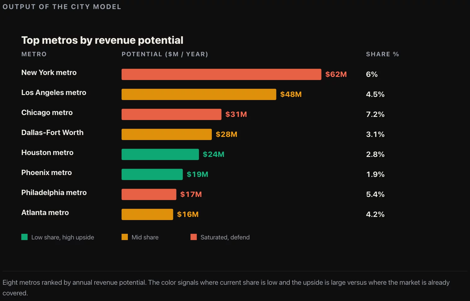
I have built two versions of this model in production. The first was for a national multi-format retailer that needed to rank 280 metropolitan areas by revenue potential per square foot of retail. The second was for a national beverage manufacturer that needed to back out its own net sales value per liter by region from the public retail audit data that was visible in trade press. Both engagements ended with a model that produced numbers the senior team trusted enough to allocate against. Neither engagement bought new data. The data was already public; the missing piece was the architecture to connect it.
The deliverable from a market sizing engagement is a single spreadsheet, never longer than four sheets, that produces a defensible per-city or per-region revenue estimate for the category the company plays in, plus the share of that revenue the company is currently capturing. Defensible means three things: every input is traceable to a public source, every assumption is named, and the model produces stable estimates when you swap any single input for its closest neighbor. The remainder of this article is how to build that spreadsheet.
What a Nielsen subscription actually buys you
A panel data subscription is not a single data product. It is a bundle of four things, and most companies who pay for one only use one or two of them. Before deciding the subscription cannot be replaced, name the parts:
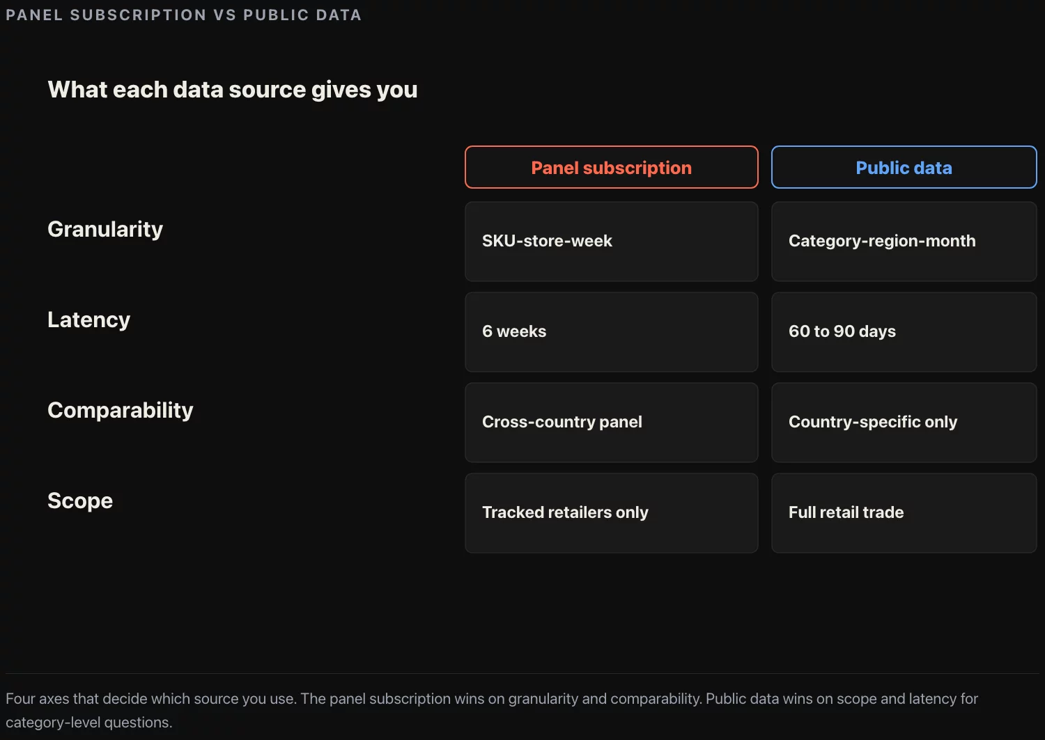
Latency. Nielsen ships data with a 2 to 6 week lag. Public retail trade data (the Census Bureau’s Monthly Retail Trade Survey, for example) ships with a 6 to 8 week lag. For board-meeting purposes the difference is not meaningful. For day-trading retail buying decisions it is. Most board questions are not day-trading questions.
Comparability. Nielsen normalizes across retailers. If Walmart and Kroger track the same SKU under different internal codes, Nielsen reconciles them. Public data does not. If you need a Walmart-vs-Kroger like-for-like comparison, panel data is the only practical source. For total-market sizing the comparability is fine because both retailers’ revenue rolls up to the same NAICS category.
Scope. Nielsen covers measured channels only. The 15% to 25% of category sales that go through unmeasured channels (independent retail, food service, direct-to-consumer for some categories) are invisible to the panel and have to be estimated separately. Public data, applied carefully, captures these.
If your strategy question is total-market sizing, share-of-category, or geographic potential ranking, public data does 80% of the work and the missing 20% is a separately answerable problem. If your question is SKU-level competitive intelligence, panel data is irreplaceable and the rest of this article does not apply to you.
The three public datasets that get you to 80%
Three datasets, all free, all updated monthly or quarterly, all accessed by API or CSV download. Together they recreate the spine of what a panel subscription gives you for total-market sizing.
Census Bureau population and income. The American Community Survey publishes population, per-capita income, and household income by metropolitan statistical area, with a 12-month rolling estimate updated quarterly. The data is granular enough to support a city-by-city model down to the 380 metropolitan areas with population above 50,000. For smaller cities (10K to 50K population) the Census decennial data plus the 5-year ACS estimates fill the gap. The key column is per-capita income; the secondary columns are population and median age, which proxy for purchasing power.
Bureau of Labor Statistics Consumer Expenditure Survey. The CEX publishes the share of household spending by category, broken out by income quintile, household composition, and region. The data answers the question “what share of a $60,000 household’s annual spending goes to food at home, vs. away from home, vs. apparel, vs. household appliances.” This is the input that converts an income estimate into a category-revenue estimate. The CEX is updated annually and is the most under-used public dataset in market sizing work. The reason it is under-used is that the data structure is awkward; the reason it is good is that the underlying survey is the same one the Bureau uses to set the CPI basket weights, which means it is methodologically robust and defensible in a board meeting.
Census Bureau Monthly Retail Trade Survey. MRTS publishes monthly retail sales by NAICS category at the national level, and quarterly by Census region. The data is what you cross-check your bottom-up city model against: if your bottom-up sum of city-level category revenue does not match the MRTS national figure within ten percent, you have a calibration problem, and you fix it before you ship the model.
The three datasets together are the spine. Layered on top are five or six secondary sources depending on category: state alcohol board sales data for beverages, USDA grain consumption for packaged food, ITA import data for goods with meaningful international supply, the Federal Reserve’s distance-to-work commuting data for retail trade area modeling. Each one is a category-specific patch on the spine; none of them is required for the basic model.
The city-level revenue model
The first model you build is bottom-up: estimate the category revenue in each city, sum to a national figure, calibrate against the MRTS national number, then use the per-city figures for ranking and prioritization.
Step 1: absolute spending per city. Multiply population by per-capita income, then by the share of income that households spend (as opposed to save or pay in taxes). For most US metropolitan areas this share is between 65% and 78%, varies with median income, and is published in the BLS CEX. The output is total household spending in the city, in dollars per year.
Step 2: category share of spending. Multiply by the share of household spending that goes to your category. For food at home this is roughly 7% to 9% of total household spending. For beer it is 0.6% to 0.9%. For household appliances it is 1.5% to 2.5%. Pull the share from the CEX, segmented by income quintile so the share is income-appropriate for the city.
Step 3: adjustment for missing inputs. Cities with population under 50K are missing from the ACS metropolitan-area tables. For those cities, estimate per-capita income from the parent state’s per-capita income, adjusted for the city’s distance from the nearest metropolitan center. The closer to the center, the closer to the metropolitan income; the farther, the closer to the rural state average. The interpolation is linear in log-distance and produces stable estimates for cities between 10K and 50K. Below 10K population the model error grows large enough that the right move is to roll the smaller cities into a “rest-of-state” aggregate rather than estimate them individually.
Step 4: company potential. Multiply by your target market share. For a brand that is the regional leader this is 25% to 40%; for a challenger it is 5% to 15%. The target is not the current share; it is the share you would hold if the city were saturated. The difference between current and target is the growth opportunity per city, which is the actual deliverable.
Step 5: B2B adjustment. For categories where business-to-business demand is meaningful (office supplies, food service, equipment), add the B2B layer on top. The marketplace I worked with used 25% as a fixed B2B share of total category sales in cities where they had a B2B sales motion, and zero elsewhere. The B2B share is the part of the model that has the weakest public data backing, and it is the part the model is most sensitive to. Be conservative.
The output of the chain is a per-city annual revenue potential figure, in dollars, for both consumer and B2B segments, with the share of the city’s total category revenue that the company is currently capturing. The model fits in one spreadsheet. The longest part of building it is locating the CEX share-of-spending number for the specific category, which usually requires reading 30 pages of BLS methodology and finding the right table.
Reverse-engineering manufacturer NSV from retail audit data
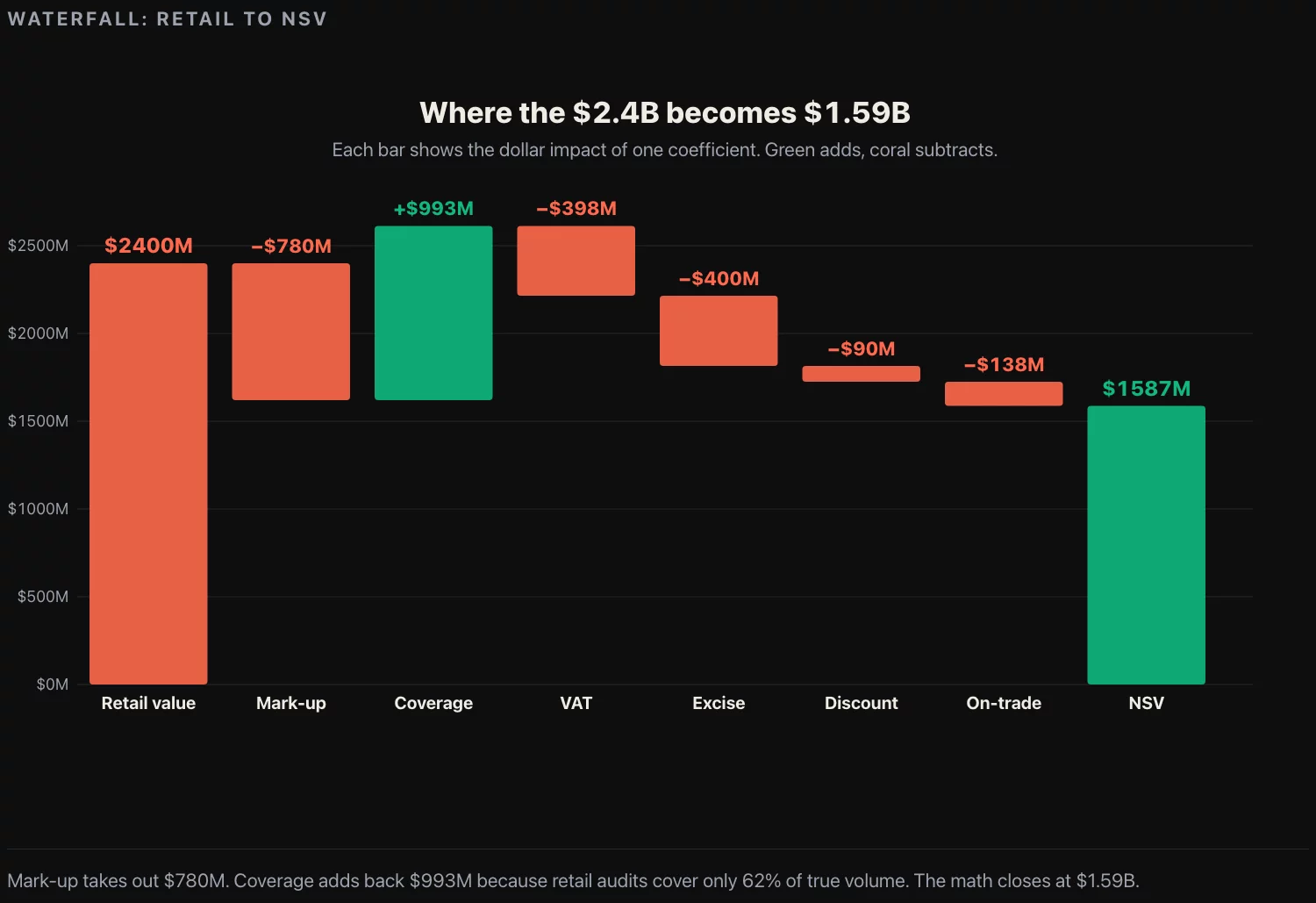
A second use case is the reverse problem. The company is a manufacturer, not a retailer. The board meeting needs the company’s net sales value per region, which is what the company sees, but the visible market data is retail audit data, which is what the retailer sees. The two numbers are different by a factor that depends on margins, excise taxes, coverage gaps, on-trade vs. off-trade splits, and promotional discounts. The factor is non-trivial; for most consumer categories it is between 0.30 and 0.55, meaning a manufacturer’s NSV is somewhere between 30% and 55% of the retail-audit revenue for the same volume.
The chain to back out NSV from retail audit numbers is:
| Coefficient | Source | Typical range |
|---|---|---|
| Retail mark-up | Trade press, retailer margin disclosures | 1.40 to 1.55 |
| Coverage adjustment (panel’s share of total channel) | Panel methodology disclosure or estimate | 0.55 to 0.70 |
| VAT (where applicable) | Regulatory | Fixed by jurisdiction |
| Excise per unit | Regulatory | Fixed by jurisdiction |
| Promotional discount | Retailer agreements, estimate | 3% to 8% |
| On-trade vs off-trade split | Trade association | Category-dependent |
Each coefficient is a row in the model. Each row has a citation. The final NSV figure is sensitive to the assumed mark-up and the assumed coverage; both are the rows the board will scrutinize, so each one carries a sensitivity column showing what NSV would be at the high and low ends of the range. A model that does not carry sensitivity columns will lose its credibility on the first slide.
The reason this matters in a fractional CDO engagement is that the operating company is usually paying for the retail audit subscription primarily to back out its own NSV by region, which it could do from public data with sensitivity columns at a tenth of the cost. The audit subscription is justified on other grounds (competitor SKU tracking, weekly granularity), but the NSV-by-region use case is the one that gets quoted first and is the one that does not actually need the subscription.
Three estimation traps
Three traps catch every first-time market sizing model. Each one collapses the model’s credibility in the board meeting if it is not handled before the meeting.
Trap one: averaging at the wrong level. Per-capita income for a metropolitan area is a mean, not a median. The mean is pulled up by a small number of high earners and overstates the spending power of the median household. For market sizing in categories where the median household is the buyer (groceries, mass-market apparel, household appliances), use median household income, not per-capita income. For luxury categories (premium spirits, luxury goods) use mean income. The choice depends on whose wallet the category lives in, and the model is sensitive to it: switching from mean to median can move the city-level estimate by 15% to 25% depending on the city’s income distribution.
Trap two: linear extrapolation across income tiers. A household at $200K does not spend twice the share on groceries that a household at $100K does. The CEX share-of-spending tables are non-linear; high-income households spend a smaller share of income on basics and a larger share on services and savings. If the city’s median income is in a different quintile from the national median, pull the CEX share for that quintile, not the national share. The model that uses the national share for all cities will overstate revenue in low-income cities and understate it in high-income cities, both in directions that make the per-city ranking unreliable.
Trap three: ignoring channel coverage gaps. Public retail trade data covers the formal retail channels reasonably well. It covers informal channels (independent retail, secondhand, gray market, direct-to-consumer for newer categories) poorly. For some consumer categories the informal channel is 15% to 30% of total volume. If the model ignores it, the bottom-up sum will match the MRTS national figure (because both ignore it) but will underestimate true category size by the size of the informal channel. The fix is to estimate the informal share from category-specific sources (trade association estimates, IRS estimates of gray-market goods, USDA estimates for food) and add it as a separate line. Be explicit about the line; do not bake it into the formal channel numbers.
The three traps are why first-pass market sizing models look reasonable and produce wrong decisions. Each one has a public-data fix that takes an extra hour to build into the model. The hour is worth it.
Calibration: how you know the model is right
A bottom-up city-by-city model is only credible if its national sum matches an independent national estimate within a tolerance. The tolerance is 10% on the first pass and 5% on the published version. The independent national estimate is the MRTS for the relevant NAICS, summed for the year, or the trade association’s national volume estimate where MRTS does not have the right category granularity.
Calibration is the step most first-pass models skip. The bottom-up sum produces a national figure of, say, $48 billion. The MRTS gives $52 billion. The 8% gap is acceptable on a first pass but the model owner should be able to explain which coefficient in the chain is most likely producing it. The standard explanation is the share-of-spending coefficient: if the CEX share is 1.5% but the bottom-up implies an effective share of 1.4%, the model is undercounting by 7%, which approximately matches the gap. Adjusting the share-of-spending coefficient up to 1.5% (with the citation) closes the gap and is defensible.
The version of the model that ships to the board carries the gap and the explanation. A model with a 1% gap and no explanation is less credible than a model with a 4% gap and a one-sentence reason. The reason is what makes the model auditable.
What to do this week
If you are about to build the first version of a market sizing model and want to start before you have approval to subscribe to anything, three actions before next Tuesday.
Pull the ACS metropolitan-area table from the Census Bureau API for population, median household income, and median age. Save it as a flat CSV. Pull the BLS CEX share-of-spending table for the most recent year for the highest-level category that contains your product. Save that as a flat CSV. You now have the two inputs for a working national model, before you have written any model code.
Pick five metropolitan areas at the high, median, and low ends of the population distribution. For each, build the four-step chain manually in a spreadsheet. Sum the five and project to a national figure by extrapolating from population. Compare the projection to the MRTS national figure for the same year. If the gap is within 25%, the methodology is going to work. If the gap is larger, the share-of-spending coefficient or the population coverage is wrong and the next hour is finding which.
Identify the one slide in the next board meeting that needs a market sizing number. Ask the strategy VP what tolerance they need on it. If the tolerance is plus-or-minus 20%, the public-data model will ship and the panel subscription is not needed for this meeting. If the tolerance is plus-or-minus 5%, neither the public-data model nor the panel subscription will get you there on the first pass, and the answer to the meeting is a range with a sensitivity analysis rather than a point estimate. Either way the next move is the same model, sized to the tolerance.
Three actions, two afternoons. They do not produce the market sizing. They produce the diagnostic that tells you whether the sizing is a model problem or a subscription problem. In my experience it is a model problem 80% of the time, and the model takes two weeks. The subscription would have taken two quarters of procurement and two analysts of training time. The board meeting is on Friday.
![[REVIEW] Looker Studio vs Power BI 2026](https://valiotti.com/wp-content/uploads/2026/06/looker-studio-vs-power-bi-2026-hero-768x512.png)