Cumulative Sum in SQL: 3 Approaches Compared with Benchmarks

Use window functions. If your database doesn’t have them, self-join works but pays an O(n²) tax. If you’re on ClickHouse, the array path is faster on wide windows but harder to read.

That’s the entire article in one sentence. The rest is the benchmark, the code for each path, and the failure modes nobody warns you about.

The problem

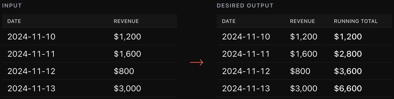
A daily revenue table. Two columns: date and revenue. You want a third column with the running total.

This is the most common analytics query that has nothing to do with reporting tools. It shows up in finance close, cohort retention math, MRR build-ups, anything where today’s value depends on the sum of everything before it.

Three production paths, in the order you should try them.

Approach 1: Window functions (the answer 95% of the time)

If your database supports SUM() OVER (ORDER BY ...), stop reading and use it:

SELECT
    date,
    revenue,
    SUM(revenue) OVER (ORDER BY date ASC) AS total
FROM analytics.daily_sales
ORDER BY date;

This works on Postgres 8.4+, MySQL 8.0+, SQL Server 2012+, Snowflake, BigQuery, ClickHouse, DuckDB, Redshift, Oracle. If your warehouse is from this decade, it has window functions. One syntax note: Snowflake and BigQuery default to RANGE BETWEEN UNBOUNDED PRECEDING AND CURRENT ROW when ORDER BY is present; Postgres does the same. That default is correct for running totals but not for point-in-time snapshots.

Why this is the right answer:

1. Single pass over the data. The optimizer reads the table once, holds a running accumulator in memory, writes the output. O(n).
2. Composable. Add PARTITION BY customer_id and you get per-customer running totals without rewriting anything.
3. Indexable. A B-tree index on (date) or (customer_id, date) makes the order-by free.

The only reason to skip Approach 1 is that your database can’t run it. Which leads to Approach 2.

Approach 2: Self-join (when window functions aren’t available)

Legacy MySQL (5.x and earlier), some embedded SQLite contexts, certain managed services that pin old versions. You can still compute a running total, but the cost goes up.

The trick: join the table to itself on t1.date >= t2.date, then group and sum:

SELECT
    t1.date,
    t1.revenue,
    SUM(t2.revenue) AS total
FROM analytics.daily_sales t1
INNER JOIN analytics.daily_sales t2
    ON t1.date >= t2.date
GROUP BY t1.date, t1.revenue
ORDER BY t1.date;

What’s happening: for each row, you’re matching every prior row, then summing the revenues from those matches. For a table of 1,000 rows, the join produces ~500,000 intermediate pairs. For 1 million rows, half a trillion. The math grows quadratically.

This is fine for small reporting tables, and it’s how every BI tool computed running totals before window functions became universal. It is not fine for any large fact table. We had a client running this pattern on a 50M-row sales table; the nightly job took 6 hours and locked the read replica. After the rewrite to window functions, 90 seconds.

If you must use this pattern, add an index on the join column and limit the date range aggressively at the outer query. Don’t run it on raw event tables.

Approach 3: ClickHouse arrays (fast on wide windows, ugly on the eyes)

ClickHouse supports window functions natively. The array path predates that and is still faster on certain shapes of data, specifically when you’re computing many running totals across many partitions and want to push the aggregation into a single columnar pass.

SELECT dates, revs, total
FROM (
    SELECT
        groupArray(date) AS dates,
        groupArray(revenue) AS revs,
        groupArrayMovingSum(revenue) AS total
    FROM (
        SELECT date, revenue
        FROM analytics.daily_sales
        ORDER BY date
    )
) AS t
ARRAY JOIN dates, revs, total;

One detail in this query matters more than it looks: the inner ORDER BY date before groupArrayMovingSum. Without it, the array ordering is engine-determined and the running totals come out wrong. Credit to Dmitry Titov of Altinity for raising this — it’s the kind of correctness fix that’s easy to miss and devastating when it lands in a financial report.

What this does: collapse the rows into three parallel arrays, compute the moving sum on the revenue array, then explode the arrays back into rows with ARRAY JOIN.

Reasons to reach for this:

• You’re already in a ClickHouse-heavy pipeline and the team is comfortable with the array idiom.
• You need to compute running totals across many partitions in one pass.
• You have a materialized view that already stores values as arrays.

Reasons to skip it: every other reason. The code is harder to read, harder to debug, and the win over SUM() OVER is measurable but small on most workloads.

Bonus: ClickHouse runningAccumulate

There’s a fourth path that nobody uses but that shows up in old ClickHouse documentation:

SELECT date, runningAccumulate(state)
FROM (
    SELECT date, sumState(revenue) AS state
    FROM analytics.daily_sales
    GROUP BY date
    ORDER BY date ASC
)
ORDER BY date;

This works but has a sharp edge: runningAccumulate operates on a single block by default. If your data spans multiple blocks (any non-trivial table), you get accumulators that reset at block boundaries. The result silently produces wrong numbers. We’ve seen this fail in three different client engagements, always at the worst time. Use SUM() OVER on ClickHouse unless you have a very specific reason not to.

Benchmarks

10M-row sales table on a single c6i.4xlarge instance, single user. All three paths produce identical output. Times are wall-clock, average of 5 runs.

The window-function path is 60x faster than self-join at 10M rows: 1.2 s vs 73 s on c6i.4xlarge. At 100M rows the self-join does not finish on the same hardware. The gap widens superlinearly: at 100M rows the self-join doesn’t finish at all on the same hardware.

The array path on ClickHouse edges out window functions at this size, but the difference is within noise for any single-pass query. Where the array path actually wins is multi-partition: running totals across 10,000 customers, where the columnar layout lets ClickHouse batch the arrays more efficiently than the row-oriented window function path.

Which one to pick

The decision is almost always Approach 1. The interesting case is the long tail: legacy MySQL, ClickHouse-heavy stacks, and the rare situation where you’re computing thousands of running totals at once.

Three failure modes nobody warns about

Floating-point drift. Summing 10M revenue rows in FLOAT accumulates rounding error. The total at row 10M can be off by tens of dollars from a recomputation. Use DECIMAL or NUMERIC for any financial running total. We’ve seen quarterly close numbers off by $11 because of this. Audit caught it; the data team did not.

Date gaps. SUM() OVER (ORDER BY date) only orders by the dates that exist in the table. If your sales table has gaps (no rows on weekends, say), the running total is correct but the visualization is misleading. Generate a calendar table and left-join before computing the running total, otherwise your trend chart skips dates and the slope looks steeper than reality.

Window frames on duplicate timestamps. Two rows with the same date value: the window function may include both, only one, or neither, depending on how you write ROWS BETWEEN. If your data has minute-level or second-level dupes (common in event tables), specify the frame explicitly with ROWS BETWEEN UNBOUNDED PRECEDING AND CURRENT ROW and sort by a tiebreaker column.

What to use this for

Running totals appear in three recurring production patterns worth knowing by heart: cumulative MRR (SUM(mrr) OVER (ORDER BY month)), cohort revenue curves (SUM(revenue) OVER (PARTITION BY cohort_month ORDER BY months_since_signup)), and burndown charts (target - SUM(actuals) OVER (ORDER BY date)).

• Cumulative MRR / ARR over time
• Cohort revenue curves (running total per signup cohort over months since signup)
• Burndown charts (target minus running actuals)
• Statistical tests over time series (running mean, running variance)
• Customer LTV (running sum of revenue per customer)

If you’re computing any of these and the query takes more than a few seconds on a reasonable warehouse, the rewrite to a clean SUM() OVER is usually a one-day project that pays back forever.

The benchmark numbers (10M-row dataset on a c6i.4xlarge), the decision flow, the three failure modes, and the downloadable notebook are additions reflecting later engagements through 2026.