Exporting Jupyter Notebooks to PDF: Three Paths and the One That Actually Works for Reports

Most data analysts know how to write a Jupyter notebook. Fewer know how to ship one. The handoff problem is real: a notebook full of cells, code, prints, and inline plots reads fine to the analyst who wrote it and badly to the stakeholder who has to extract a conclusion from it. The usual fix is to copy the charts into Google Slides, paste the numbers into an email, and lose the reproducibility along the way.

Exporting the notebook directly to PDF is the better fix, when it works. The reader gets a clean document with charts, tables, narrative, and no scrolling. The analyst keeps the source notebook as the canonical artifact. Nothing has to be rebuilt manually for the next iteration.

The catch is that “export to PDF” in Jupyter is not one feature. It is three or four overlapping mechanisms, each with its own install requirements and its own failure modes. This piece walks through the three I would actually use, the one I default to, and the small tricks that make the output look like a report instead of a notebook printout.

The three paths, ranked by install cost

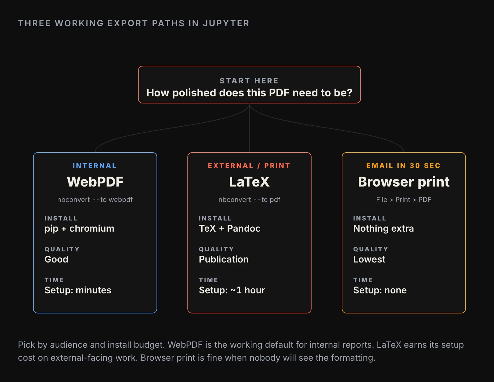
The three working export paths in Jupyter all run through the same command-line tool, nbconvert, but they take different conversion routes underneath. Picking the right path is mostly a question of how much install you are willing to do and how polished the output has to be.

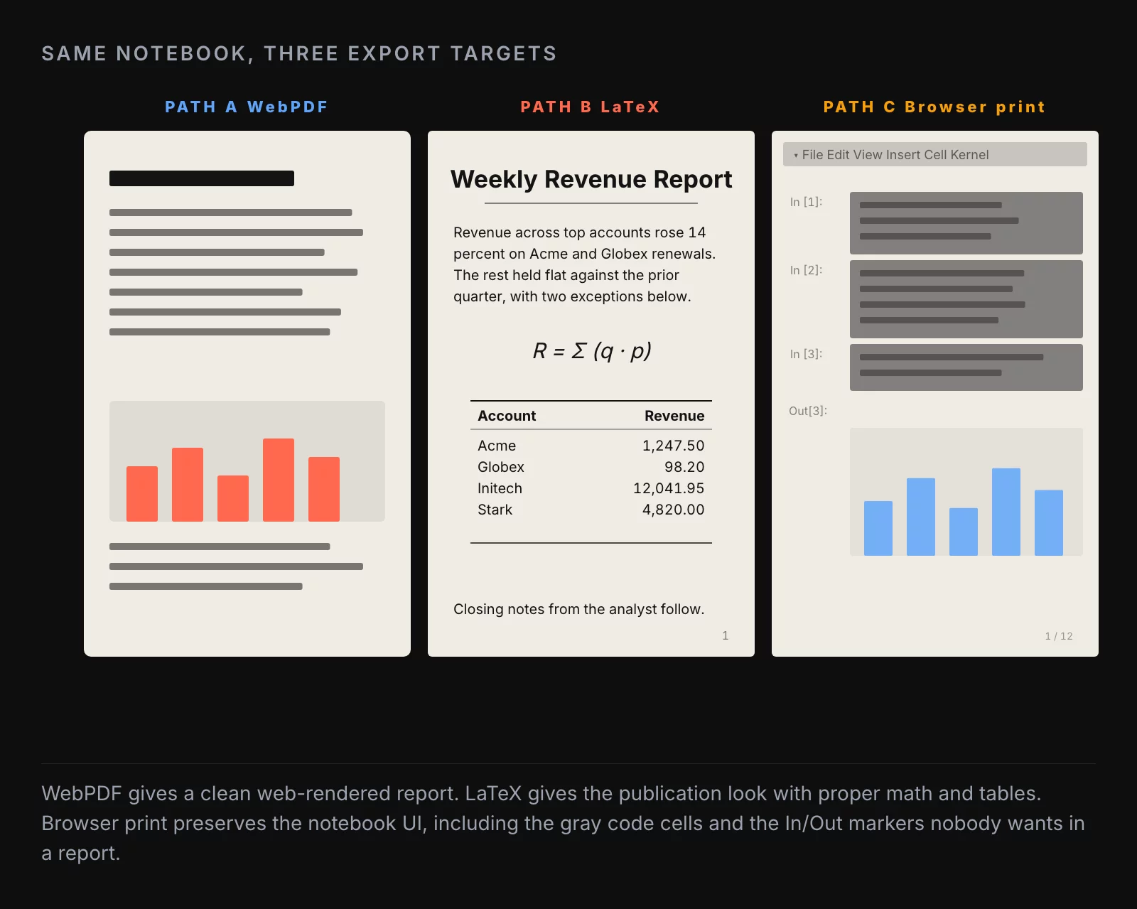
Path A: WebPDF (headless Chromium). Fastest to set up. nbconvert renders the notebook to HTML, then a headless Chromium prints the HTML to PDF. Install is a single pip install nbconvert[webpdf] plus a one-time playwright install chromium. Output looks like a screenshot of the notebook with cleaner page breaks. Good for internal reports, weekly analytics, anything where the audience is going to read the PDF on a screen.

Path B: LaTeX (the canonical path). Highest quality output. nbconvert runs the notebook through Pandoc, then a TeX engine compiles a real LaTeX document into a PDF. Install is heavy: Pandoc plus a full TeX distribution (TeX Live on Linux, MacTeX on macOS, MiKTeX on Windows). The first install can take an hour and several gigabytes of disk. The output is publication-quality, with proper kerning, math typeset by TeX, and a layout that survives printing. Use this when the PDF is going to a client, a paper, or anywhere it might get printed and bound.

Path C: Browser print. Lowest effort, lowest quality. Open the notebook in the browser, hit File → Print Preview, then print to PDF. Works without installing anything extra. The output is a screenshot of the notebook UI, complete with the gray code cell backgrounds and the In/Out markers. Use this when you need a PDF in the next thirty seconds for an email and the formatting does not matter.

In practice, almost every analyst I work with starts on Path C (because they have not heard of the other two), graduates to Path A when they get tired of the gray code cells, and only adopts Path B if they have a regular client-facing reporting workflow. Path B is the right answer for external reporting and overkill for everything else.

Path A: WebPDF, the working default

This is the path I default to. Install is fast, output is clean, and the failure modes are easy to debug.

pip install "nbconvert[webpdf]"
playwright install chromium

To export:

jupyter nbconvert --to webpdf --allow-chromium-download my_notebook.ipynb

The --allow-chromium-download flag is only needed the first time, while Playwright pulls down its Chromium binary. After that the flag is optional.

The output is a PDF named my_notebook.pdf in the same directory as the notebook. Page breaks land where Chromium picks them, which is usually fine for analytical reports but can split a plot across two pages if the plot is taller than half a page. The fix is to size the plot deliberately in the notebook, or to add a manual

The other useful flag is --TemplateExporter.exclude_input=True, which hides all the input cells and keeps only the markdown narrative and the cell outputs. This is the difference between “a notebook printed to PDF” and “a report.” For any external-facing PDF, the input-cell exclusion is non-negotiable. The stakeholder does not want to see the pandas import statement on page one.

jupyter nbconvert --to webpdf --TemplateExporter.exclude_input=True my_notebook.ipynb

The output now contains only the markdown text, the plots, the table outputs, and any explicit print statements. It reads like a report.

Path B: LaTeX, the canonical path

The LaTeX path produces the best-looking output and demands the most setup. The trade-off is worth it for any work going to a paying client or to a context where the PDF might be printed and read on paper.

The dependencies are:

• Pandoc (the document converter Jupyter delegates to)
• A TeX distribution (TeX Live, MacTeX, or MiKTeX)
• nbconvert (the Jupyter conversion CLI)

On macOS, the install is roughly:

brew install pandoc
brew install --cask mactex
pip install nbconvert

On Ubuntu or Debian:

sudo apt-get install pandoc texlive-xetex texlive-fonts-recommended texlive-plain-generic
pip install nbconvert

The TeX install is the slow part. MacTeX is around four gigabytes. The Ubuntu packages can be done with the slimmer texlive-xetex set if disk is tight, but the slim set will sometimes fail to compile a notebook that uses an unusual symbol or a non-Latin character. If the budget is there, install the full TeX distribution.

To export:

jupyter nbconvert --to pdf --TemplateExporter.exclude_input=True my_notebook.ipynb

The output PDF has the LaTeX look: serif body type, justified paragraphs, proper math layout, and a clean header treatment. Equations written in markdown cells using LaTeX syntax ($sum_{i=1}^{n} x_i$) compile correctly. Tables converted to markdown format render with the LaTeX booktabs style, which looks substantially more professional than the default HTML table style.

The most common failure mode on the LaTeX path is a missing TeX package, surfaced with an error like ! LaTeX Error: File 'something.sty' not found. The fix on TeX Live is tlmgr install something. On MacTeX it is sudo tlmgr install something. The error message names the missing file; the package name is usually the filename without the extension.

The tabular-data trick: convert pandas to markdown before export

Both Path A and Path B handle pandas DataFrames poorly by default. The notebook displays a styled HTML table; nbconvert converts that HTML to either a screenshot-ish block (WebPDF) or a plain LaTeX table (LaTeX path), and neither result is what you actually wanted.

The reliable workaround is to convert the DataFrame to a markdown table inside the notebook, and let the export pipeline treat it as text:

from IPython.display import Markdown, display

def df_to_markdown(df):
    fmt = ['---' for _ in range(len(df.columns))]
    df_fmt = pd.DataFrame([fmt], columns=df.columns)
    df_formatted = pd.concat([df_fmt, df])
    display(Markdown(df_formatted.to_csv(sep="|", index=False)))

summary = round(data.describe(), 2)
summary.insert(0, 'metric', summary.index)
df_to_markdown(summary)

The output renders as a clean markdown table in the notebook and exports as a properly formatted table in the PDF on both paths.

The one gotcha is that the DataFrame index does not survive the conversion. If the index is meaningful (a column of metric names, a date index), copy it into an explicit column with df.insert(0, 'index_name', df.index) before passing the DataFrame to the function above. Forgetting this step is the most common cause of “where did my row labels go” tickets after the first PDF export.

The image trick: write to disk, then display

Plotly figures, Bokeh figures, and a few other interactive chart libraries do not survive the notebook-to-PDF conversion. The interactive widget cannot render in a static PDF, and nbconvert either drops the chart entirely or inserts a placeholder.

The fix is to write the figure to disk as a static image and re-display the image inside the notebook:

import plotly.express as px
from IPython.display import Image

fig = px.scatter(
    data.query("year == 2007"),
    x="gdpPercap", y="lifeExp",
    size="pop", color="continent",
    log_x=True, size_max=70,
)
fig.write_image('figure_1.jpg')
Image(filename='figure_1.jpg', width=1000)

The write_image call requires the kaleido package for Plotly (pip install kaleido). Once it is installed, the figure renders to a JPG (or PNG, if you prefer) and the subsequent Image call displays it inline. The PDF export captures the static image cleanly on both paths.

The same pattern works for any chart library that supports a static-export method: Altair has chart.save('file.png'), Bokeh has bokeh.io.export_png, matplotlib obviously needs no help because it is already static.

Common pitfalls and how to fix them

A short list of the failure modes that eat the most time.

The TeX install fails or is missing a package. The error message names the missing file. Run tlmgr install to add it. If tlmgr is not on the path, the TeX distribution is installed but the binaries are not in your shell PATH; restart the terminal or add /Library/TeX/texbin (macOS) or /usr/local/texlive/2024/bin/x86_64-linux (Linux) to your $PATH.

The PDF has a page break in the middle of a plot. Either resize the plot to be shorter than half a page, or add an explicit page break in the markdown above the plot with

Tables look like screenshots instead of typeset tables. You exported the HTML representation of the DataFrame instead of converting it to markdown first. Use the df_to_markdown function above.

Math equations render as plain text. The markdown cell needs explicit LaTeX-style math delimiters: $inline$ for inline math and $$display$$ for display math. The WebPDF path handles math through MathJax; the LaTeX path renders it natively.

The code cells show up in the output. You forgot --TemplateExporter.exclude_input=True. Add it to the command, or set it in a jupyter_nbconvert_config.py to make the exclusion the default.

The PDF is missing a chart that worked in the notebook. It is almost certainly a Plotly or Bokeh figure that did not get rendered to a static image. Apply the image trick above.

Special characters render as boxes or question marks. The slim TeX install does not have the font that supports the character. Install the full TeX distribution, or replace the character (a stray em-dash, an unusual unicode symbol) with a supported equivalent.

A working checklist before you ship the PDF

A list to run before you email the document:

• Code cells excluded with --TemplateExporter.exclude_input=True
• Tables converted to markdown via the df_to_markdown helper, not left as HTML DataFrame output
• All Plotly and Bokeh figures written to disk and re-displayed as static images
• No chart split across a page break (resize, or insert a manual page break)
• Math equations wrapped in $...$ or $$...$$
• Markdown headings used in a sensible hierarchy (one H1 for the title, H2 for sections, H3 for subsections)
• Filename is human-readable (weekly_revenue_review_2026_05_26.pdf, not Untitled (3).pdf)
• The PDF opens cleanly in a viewer that is not Chrome (test in Preview or Acrobat to catch font issues)

A notebook that passes that list will produce a PDF a stakeholder will read. The Path A version takes around five minutes to set up the first time and seconds to run thereafter. The Path B version takes longer to set up and produces an output worth the install cost on any external-facing report.

Further reading

• 10 Dashboard Design Rules, 6 Years Later, the layout principles the markdown-table trick is in service of
• Choosing Fonts for Data Visualizations, the font choices that come back the moment you start customizing the LaTeX template

About the author

Nick Valiotti is the founder of Valiotti Data. 15+ years building analytics infrastructure for SaaS, marketplaces, and consumer subscription. 50+ production deployments across BigQuery, Snowflake, dbt, Metabase, and modern BI stacks. Author of two books on data strategy. LinkedIn · Discovery call.